Recently, I was trying to classify images of birds by using machine learning technology. The most familiar deep learning library for me is the mxnet, so I use its python interface to build my Birds-Classification-System.
For having not sufficient number of images for all kinds of bird, I just collect three types of them: “Loggerhead Shrike”, “Anhinga”, and “Eastern Meadowlark”.
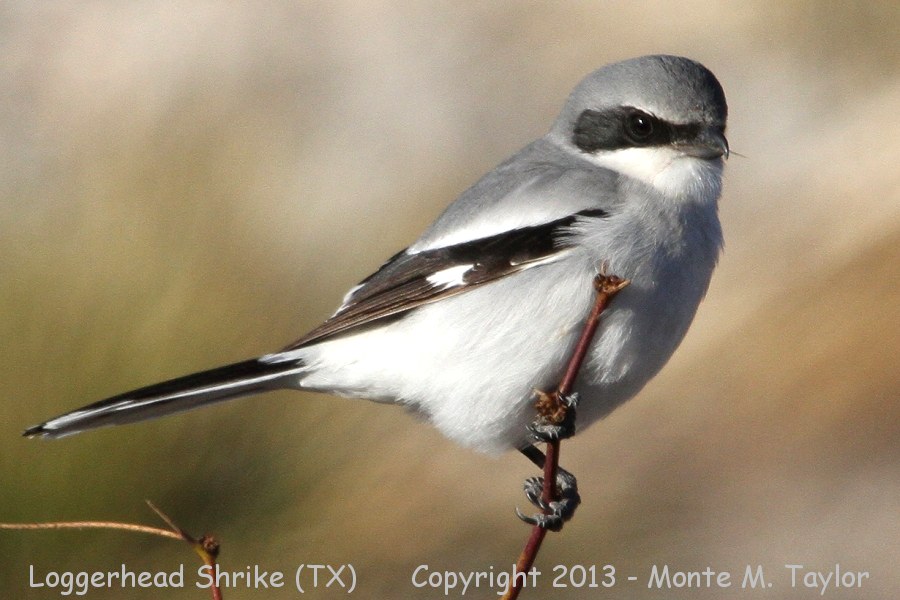 Loggerhead Shrike Loggerhead Shrike |
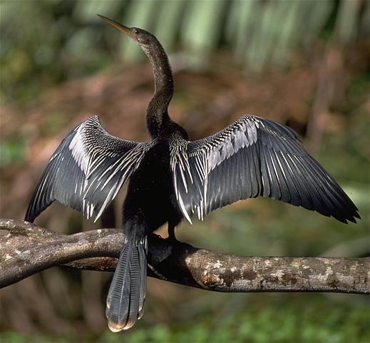 Anhinga Anhinga |
 Eastern Meadowlark Eastern Meadowlark |
After collecting more than 800 images of the three kinds of bird, I started to write my python code by learning the “Handwritten Digital Sample” of mxnet step by step.
Firstly, using PIL (Python Image Library) to preprocess these images – chop them from rectangle to square with 100 pixels length of edge:
edge = 100
......
def process_image(file_name):
    img = Image.open(file_name)
    tp = img.getbbox()
    width = tp[2]
    height = tp[3]
    if (width > height):
        sub = width - height
        img = img.crop((sub / 2, 0, height + sub / 2, height))
    elif (height > width):
        sub = height - width
        img = img.crop((0, sub / 2, width, width + sub / 2))
    img.thumbnail((edge, edge), Image.NEAREST)
    return img
Then put all images into a numpy array and label them:
images = np.array([])
labels = np.array([])
nr_images = 0
......
      for file in files:
        img = process_image(bird_dir + file)
        global images, labels, nr_images
        if array.shape == (edge, edge, 3):
          images = np.append(images, np.asarray(img))
          labels = np.append(labels, lab)
          nr_images = nr_images + 1
Now I can build the Convolutional Neural Network model easily by using the powerful mxnet. The CNN will slice all pictures to 8×8 pixels small chunk with 2 pixels step, therefore enhance the small features of these birds, such as black-eye-mask of Loggerhead-Shrike, yellow neck of Eastern-Meadowlark, etc.
def convolution_network():
    data = mx.sym.Variable('data')
    conv1 = mx.sym.Convolution(data=data, kernel=(8, 8), stride=(2,2), num_filter=8)
    bn1 = mx.sym.BatchNorm(data=conv1, fix_gamma=False, eps=2e-5, momentum=0.9, name="bn1")
    tanh1 = mx.sym.Activation(data=bn1, act_type="relu")
    flatten = mx.sym.Flatten(data=tanh1)
    fc1 = mx.sym.FullyConnected(data=flatten, num_hidden=1000)
    tanh3 = mx.sym.Activation(data=fc1, act_type="relu")
    fc3 = mx.sym.FullyConnected(data=tanh3, num_hidden=3)
    return mx.sym.SoftmaxOutput(data=fc3, name='softmax')
Training the data:
images = np.array(images).reshape(nr_images, 3, edge, edge).astype(np.float32)/255
batch_size = 200
train_iter = mx.io.NDArrayIter(images, labels, batch_size, shuffle=True)
mlp = convolution_network()
model = mx.model.FeedForward(
        ctx = mx.gpu(0),
        symbol = mlp,
        num_epoch = 40,
        learning_rate = 0.02
model.fit(
        X = train_iter,
        batch_end_callback = mx.callback.Speedometer(batch_size, 1))
Using GPU for training is extremely fast – it only cost me 5 minutes to train all 800 images, although adjusting the parameters of CNN cost me more than 3 days 🙂
Firstly I use Fully Connected Neural Network, it costs a lot of time for training but prone to overfit. After using the CNN with BatchNorm() in mxnet, the speed of training and affect of classification advanced significantly.
CNN(Convolutional Neural Network) is really a ace in deep learning area for images!